3 Descriptive Analytics for Time Series Data

3.1 Overview

For descriptive analysis, the focus was on questions such as: What is typical? How spread out is the data? What shape does the distribution have? With time series data, an additional question becomes important: When did it happen?

Time series data is a sequence of observations collected or recorded at successive points in time. Because observations are ordered chronologically, time series data provides a dynamic view of how a variable changes over time, rather than a static snapshot.

Chronological order: Observations occur sequentially over time so ordering of the data matters.
Time index: Each oberservation is associated with a specific point in time.
Dependence over time: Earlier and later observations may be related, meaning observations may not be independent.
Temporal patterns: The ordering of observations allows patterns like trend, seasonality, and short term variation to be identified.

Suppose a CFO says” “Sales dropped 15% from Q3 to Q4.”

That number by itself doesn’t necessarily mean the business suddently got worse. Maybe sales normally decline from Q3 to Q4 and this is just a regular reoccurring observation.

With time series data, there are three things to be distinguished:

Trend \(\rightarrow\) Is there a long-term upward/downward movement?
Seasonality \(\rightarrow\) Does a pattern repeat at regular intervals?
Noise \(\rightarrow\) Is a movement just short-term random variation?
Level Change \(\rightarrow\) Did the series actually shift to a different level?

3.2 Working with Lubridate

Why do dates matter in analytics? Dates can be used for several things, for example:

Time aware filtering (e.g. time based filtering), time aware grouping (group a time period), and trend/seasonality detection.
Aligning events (comparing before and afters).
Preparing for forecasting.

Dates need to actually be dates! A date stored as text like:

'2025-08-21'

is much different from an R Date object actually representing August 21, 2025. The main package used when working with dates is lubridate.

3.2.1 Parsing Dates

Parsing dates is the process of converting raw string dates to an actual date/time object, which can then be converted into useful time components. Raw string dates may not always be written in a consistent way, therefore different functions are used based on what the text format is.

ymd() when string = YEAR \(\rightarrow\) MONTH \(\rightarrow\) DAY
mdy() when string = MONTH \(\rightarrow\) DAY \(\rightarrow\) YEAR
dmy() when string = DAY \(\rightarrow\) MONTH \(\rightarrow\) YEAR
ymd_hms() when string = YEAR \(\rightarrow\) MONTH \(\rightarrow\) DAY : HH:MM:SS

Example:

ymd("2025-08-21")

[1] "2025-08-21"

mdy("08/21/2025")

[1] "2025-08-21"

dmy("21-Aug-2025")

[1] "2025-08-21"

ymd_hms("2025-08-21 14:30:00")

[1] "2025-08-21 14:30:00 UTC"

Once the date is in the correct format, R can extract pieces:

year(x) = extract year
month(x) = extract month
quarter(x) = extract quarter
wday(x) = extract weekday
hour(x) = extract hour
isoweek(x) = extract week number of year

x <- ymd_hms("2025-08-21 14:30:00")
x

[1] "2025-08-21 14:30:00 UTC"

year(x)

[1] 2025

month(x)

[1] 8

quarter(x)

[1] 3

wday(x)

[1] 5

hour(x)

[1] 14

isoweek(x)

[1] 34

Esssentially the process is raw date string → actual date/time object → useful time components

Dates can also be created from combining variables that already exist. For example if you have year = 2025 and month = 8 you can construct an actual date.

make_date() use when year/month columns exist because it avoids rounding problems associated with fractional-year representations

# Before: year and month are separate variables
txhousing |>
    select(year, month) |>
    head(2)

# A tibble: 2 × 2
   year month
  <int> <int>
1  2000     1
2  2000     2

# Create an actual date from year and month
TX <- txhousing |>
    mutate(
        date_actual = make_date(
            year = year,
            month = month,
            day = 1
        )
    )

# After: year and month have been combined into a date
TX |>
    select(year, month, date_actual) |>
    head(2)

# A tibble: 2 × 3
   year month date_actual
  <int> <int> <date>     
1  2000     1 2000-01-01 
2  2000     2 2000-02-01

3.2.2 Calendar Arithmetic

Leap years can screw up calculation of dates. For example ymd("2024-02-29") is a leap year. If you subtract five years you’d get 2019-02-29 which doesn’t exist.

d1 <- ymd("2024-02-29")

lubridate has calendar awareness operators:

d1 %m-% years(5)

[1] "2019-02-28"

ymd("2023-01-31") %m+% months(1)

[1] "2023-02-28"

3.2.3 Time Windows

Once dates are represented properly, normal comparisons work:

TX |>
    filter(
        date_actual >= as.Date("2005-01-01"),
        date_actual <= as.Date("2010-12-31")
    )

# A tibble: 3,312 × 10
   city     year month sales  volume median listings inventory  date date_actual
   <chr>   <int> <int> <dbl>   <dbl>  <dbl>    <dbl>     <dbl> <dbl> <date>     
 1 Abilene  2005     1   119  1.03e7  74200      570       3.7 2005  2005-01-01 
 2 Abilene  2005     2   130  1.18e7  74300      581       3.7 2005. 2005-02-01 
 3 Abilene  2005     3   170  1.45e7  71300      661       4.3 2005. 2005-03-01 
 4 Abilene  2005     4   171  1.64e7  80300      650       4.2 2005. 2005-04-01 
 5 Abilene  2005     5   176  1.81e7  87100      660       4.2 2005. 2005-05-01 
 6 Abilene  2005     6   230  2.41e7  92500      664       4.1 2005. 2005-06-01 
 7 Abilene  2005     7   177  1.85e7  93500      657       4.1 2006. 2005-07-01 
 8 Abilene  2005     8   216  2.41e7  97500      638       3.9 2006. 2005-08-01 
 9 Abilene  2005     9   165  1.71e7  92800      644       3.9 2006. 2005-09-01 
10 Abilene  2005    10   161  1.64e7  92300      601       3.6 2006. 2005-10-01 
# ℹ 3,302 more rows

You can also make relative windows.

For example, find the most recent date:

max_date <- max(TX$date_actual, na.rm = TRUE)
max_date

[1] "2015-07-01"

Then go five years backward:

start_5y <- max_date %m-% years(5)
start_5y

[1] "2010-07-01"

Then:

recent <- TX |>
    filter(date_actual > start_5y)

head(recent)

# A tibble: 6 × 10
  city     year month sales   volume median listings inventory  date date_actual
  <chr>   <int> <int> <dbl>    <dbl>  <dbl>    <dbl>     <dbl> <dbl> <date>     
1 Abilene  2010     8   144 17504580 122000      936       6.7 2011. 2010-08-01 
2 Abilene  2010     9   116 15475763 121300      899       6.5 2011. 2010-09-01 
3 Abilene  2010    10   111 14570529 111900      863       6.4 2011. 2010-10-01 
4 Abilene  2010    11   115 11422741  87900      851       6.4 2011. 2010-11-01 
5 Abilene  2010    12   116 15289470 118300      830       6.3 2011. 2010-12-01 
6 Abilene  2011     1    68  8834493 123300      809       6.1 2011  2011-01-01

So instead of hard-coding a five-year range, you’re saying:

Give me observations from the final five years of the dataset.

For time-series data, the standard visualization is a line chart.

The lecture calculates statewide median sales for each month:

TX |>
    group_by(date_actual) |>
    summarise(
        median_sales = median(sales, na.rm = TRUE)
    ) |>
    ggplot(aes(date_actual, median_sales)) +
    geom_line()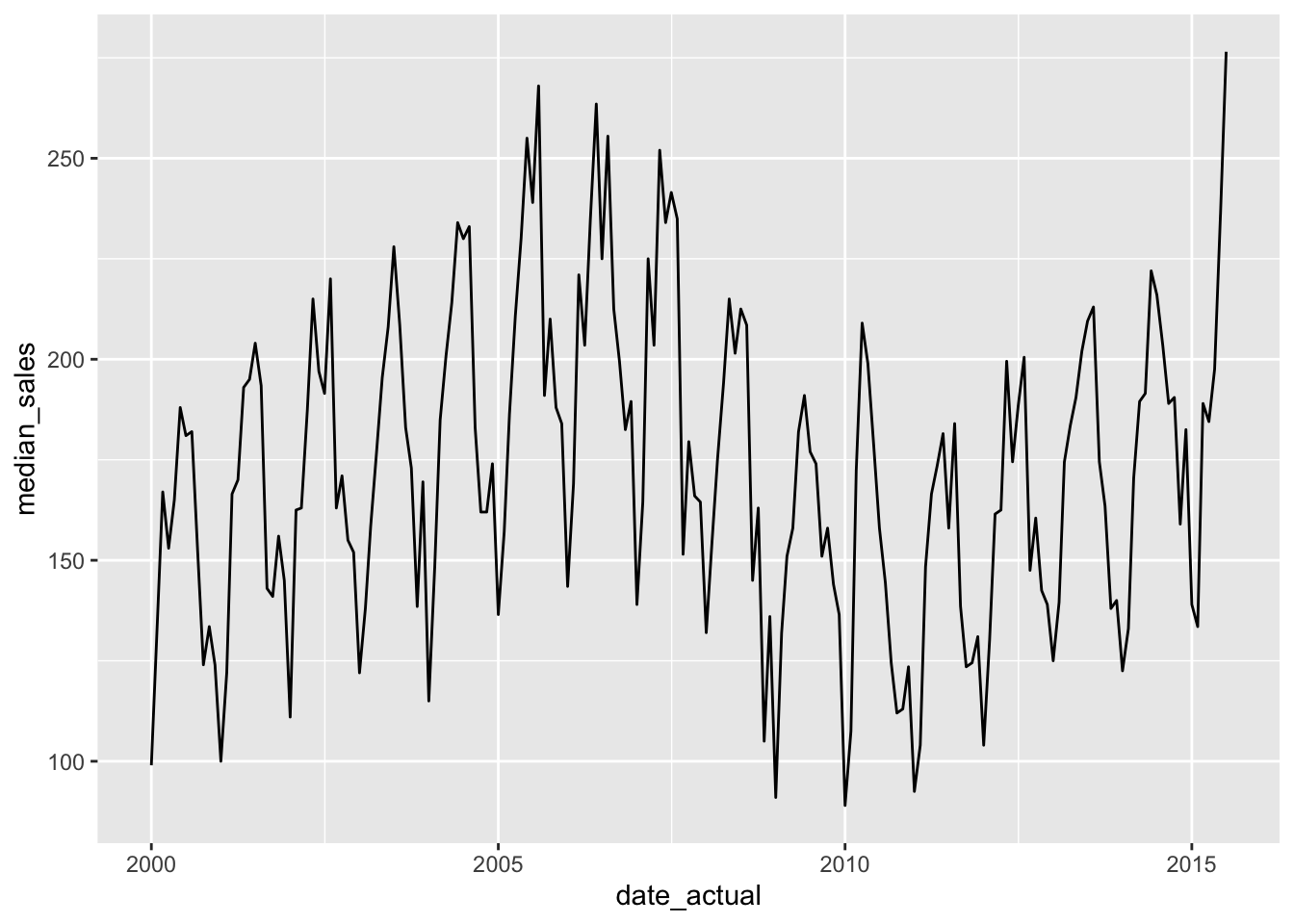

The conceptual structure is:

Date → x-axis
Value → y-axis

Connecting observations makes the evolution of the variable visible.

scale_x_date() then controls how frequently dates are displayed so that a long time horizon doesn’t produce an unreadable x-axis.

3.2.4 Seasonality

Seasonality is one of the central concepts of time series data.

Seasonality is a pattern that systematically repeats according to the calendar.

It can be viewed by:

Lines by year:

TX |>
    ggplot(aes(
        x = month(date_actual, label = TRUE),
        y = sales,
        group = year,
        color = as.factor(year)
    )) +
    geom_line()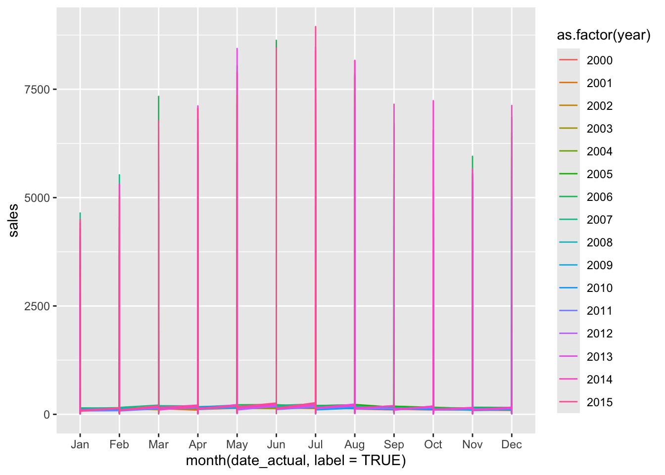

Boxplots by month

What does a typical January look like across years? What does a typical July look like?

TX |>
    ggplot(aes(
        x = month(date_actual, label = TRUE),
        y = sales
    )) +
    geom_boxplot()

Warning: Removed 568 rows containing non-finite outside the scale range
(`stat_boxplot()`).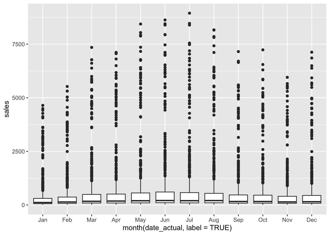

Heatmaps are another view of seasonality

   2005  2006  2007  2008 ...

Jan ■ ■ ■ ■ Feb ■ ■ ■ ■ Mar ■ ■ ■ ■ … Dec ■ ■ ■ ■

where the fill intensity represents sales.

3.2.5 Moving Averages

Month-to-month fluctuations can make the underlying trend difficult to see. A rolling average smooths those fluctuations.

monthly_sales <- TX |>
    group_by(date_actual) |>
    summarise(
        median_sales = median(sales, na.rm = TRUE)
    ) |>
    arrange(date_actual) |>
    mutate(
        moving_average = rollmean(
            median_sales,
            k = 12,
            fill = NA,
            align = "right"
        )
    )

monthly_sales

# A tibble: 187 × 3
   date_actual median_sales moving_average
   <date>             <dbl>          <dbl>
 1 2000-01-01            99             NA
 2 2000-02-01           134             NA
 3 2000-03-01           167             NA
 4 2000-04-01           153             NA
 5 2000-05-01           165             NA
 6 2000-06-01           188             NA
 7 2000-07-01           181             NA
 8 2000-08-01           182             NA
 9 2000-09-01           152             NA
10 2000-10-01           124             NA
# ℹ 177 more rows

k = 12 means a 12-observation window. Because the data are monthly, that’s a 12-month moving average.